| www.ethanwiner.com - since 1997 |
Spectrum Analyzer and Equalizer Designs
by Ethan Winer
This article first appeared in the February 1982 issue of Recording-engineer/producer magazine
A spectrum analyzer can be a powerful tool for keeping your studio well tuned. Besides its obvious uses - for adjusting octave or one-third octave room equalizers - a spectrum analyzer can also be used to check the response of a tape recorder, or even help identify the rumble frequencies in an air conditioner. Unfortunately for many studios, the high price of a commercial spectrum analyzer presents a major problem; LED versions cost many hundreds of dollars, and a good oscilloscope model can run into thousands. But once again the IC op-amp comes to the rescue, allowing construction of a sophisticated "manual" analyzer that includes a clever but unusual digital pink-noise source, all for just the cost of a few components.
Although a real-time analyzer is more convenient to use because of its simultaneous display of all frequency bands, a manually swept model is no less professional and its use follows well established practice. In fact, a continuous sweep can detect narrow peaks and dips, which would be ignored by a real-time unit with its fixed third-octave spacing.
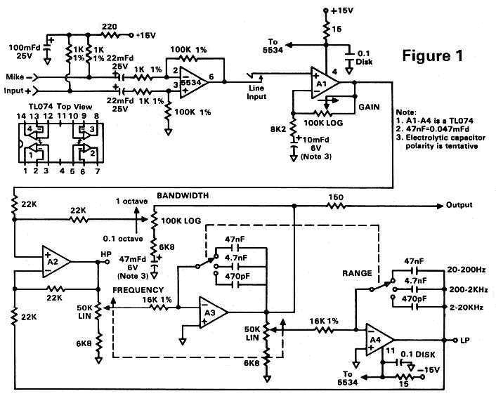
The circuit shown in Figure 1 uses only two ICs, and has a bandwidth that is adjustable from more than one octave down to a tenth of an octave. As shown, the frequency range is 20 Hz. to 20 KHz. in three bands, although a fourth subsonic band could be added to allow very low frequency analysis. A low-noise mike preamplifier is included, and a line input is also available with up to 20 dB of gain. Of course, you could use a mike preamp in your console instead, but at the expense of portability.
Selecting a suitable measuring microphone is crucial for serious room analysis, since no doubt the mike will be the weakest link in the measuring chain. First, it should be omni-directional because reflections off walls, ceilings and floors contribute greatly to the sound of a room and must be taken into account. Second, the mike element must be a small capsule condenser type, since the large diaphragm in a Neumann U-87 or an AKG C-414 is bigger than some of the wavelengths being measured causing inaccuracies at high frequencies. When cost is no object, special measuring microphones are available with really tiny elements. Although such mikes generally have a relatively low output, their frequency response is extremely flat. One possible exception is when voicing a PA system, where a typical stage mike might be a better choice. This way response errors in the mikes are included in the measurement and correction process.
I chose an AKG CK-22 capsule that fits a C451 mike, because I trust the manufacturer to give me an accurate graph of its response and because I already have the mike. No doubt other small capsule omni-directionals from Neumann and others could be used, although the AKG C451/CK22 can be reliably operated from as little as 12 V, which makes phantom powering much easier.
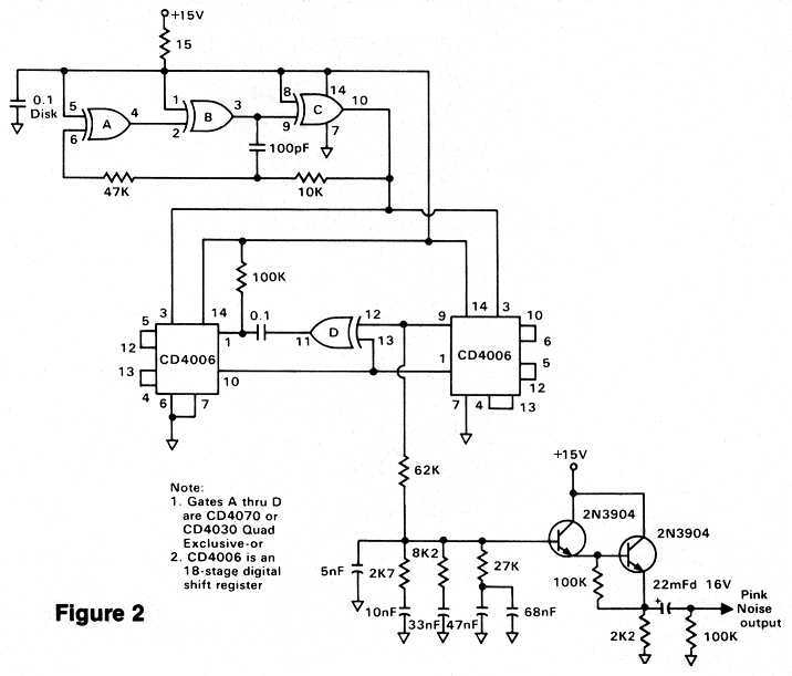
Pink noise - which contains all frequencies simultaneously - is frequently used as a signal source when measuring speakers. Many noise generator designs use a reverse biased semiconductor junction as the actual noise source. But this requires you to test many transistors, select one that produces "good" noise, and then amplify the small signal. The noise is then passed through a pink noise filter. While the circuit of Figure 2 represents a somewhat more complicated approach, the results obtained are much more predictable.
A high-frequency CMOS IC oscillator is used as a clock connected to a 31-stage digital shift register. Without getting into the gory details, this shift register is configured as a pseudo-random binary sequence generator (whew!) which, when clocked fast enough, creates extremely pure wide bandwidth white noise. White noise, however, has a rising high-end when measured on an octave basis, since every frequency is represented by the same amount of energy. In other words, the octave from 10 KHz. to 20 KHz. has twice as much energy as the octave from 5 KHz. to 10 KHz. because twice as many cycles are considered. Audio work measures energy by the octave or fraction of an octave, so a continuous 3 dB. per octave high-end roll-off of the noise is required to maintain the proper perspective. The only problem is that filters always come in multiples of 6 dB. per octave, since this is the minimum amount of attenuation obtainable with a single resistor and capacitor. Therefore, a compound filter must be designed with multiple RC networks, with each contributing a little to the overall curve as shown in Figure 2. The output of this filter must not be loaded by a low impedance, so a two transistor Darlington follower is used as an output buffer rather than a simple emitter follower. An op-amp follower could also be used, but the transistors are sufficient here.
Returning to the analyzer, a state-variable filter is used in the band-pass mode, and can be swept in three switch selected ranges: 20 to 200 Hz.; 200 Hz. to 2 KHz.; and 2 to 20 KHz. A state-variable design was chosen for several reasons: the tuning frequency can be easily varied while maintaining a perfectly uniform response, and the Q - or bandwidth - can be controlled independently. If you notice a similarity between this filter and a parametric equalizer, you won't be surprised to know that many parametrics are based on a state-variable design. Admittedly, this type of active filter is more complicated than other designs since three op-amps are required in place of the usual one. But many useful audio gadgets can be built with such a state-variable filter design, as you will see later in this article.
Referring to Figure 1, an NE5534 op-amp is used for the mike preamplifier stage because of its low input noise. Forty dB. of gain is sufficient for most microphones, since the pink noise will be played through the speakers at a moderately high level. If you can't obtain 1% resistors 5% types will do, but only if you aren't located near a radio transmitter or in a metropolitan area. The 22 uF. capacitors block the phantom power from the preamp's input, and the 100 uF. capacitor is used as a filter to remove any traces of noise on the power supply. Of course, whenever building sensitive circuits you should use a regulated power supply.
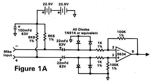
If you do not use a C451 microphone you must provide a full 48 volts as the phantom power source. Batteries of 22.5 Volts the size of a penlight cell are available at camera and Radio Shack stores, and you can use two of these wired in series. Also, you must increase the voltage rating of the input capacitor, the value of the resistors for the phantom supply, and add diodes to protect the op-amp from turn-on spikes - all of which are shown in Figure 1A.
Once the input has been sufficiently amplified, it is sent to the state-variable filter comprising op-amps A1 through A4. As with many active filters, the input is to a summing junction, or negative feedback node. Unlike most summing junctions, however, this one is at the plus input of an op-amp (A2). The feedback is still negative since an inverting stage (A3) has been placed in its feedback loop. A3 and A4 serve as integrators, with a capacitor as the feedback element; the tuning frequency is determined by the setting of the dual 50k pot, the 16k integrator resistors, and the capacitors.
The bandwidth is varied by adjusting the amount of feedback to A2's plus input and, as you might expect, the filter's gain increases along with the reduction in feedback just like a normal amplifier stage. Fortunately, this increase in gain is partially offset by the reduced bandwidth being measured, as mentioned earlier. In fact, any noise measurement or specification is meaningless if you don't know the range of frequencies being considered.
Besides being able to easily vary the Q and tune its frequency, a state-variable filter also provides a high-pass and low-pass output, and these are available at A2 and A4 respectively. A swept notch can also be achieved simultaneously, by combining the input to the filter (A1's output) with the band-pass output in a summing amp, as shown in the THD analyzer circuit in my Pre-Distortion article from the December 1981 issue of R-e/p. An ambitious builder could add the 20 dB. gain stage required, and have a super all-in-one test instrument to use in the studio.
For all of the filter components it is important to use the closest tolerance parts you can get your hands on. One-percent metal film resistors are the best, not only because of their accuracy but also for their reduced sensitivity to temperature. For this same reason, polycarbonate or mylar capacitors are the best choice for the actual filter stages. For power supply bypass disk capacitors are not only sufficient but preferred, since they possess less series inductance. Tubular types, though generally more temperature stable, are constructed of long strips of foil which when rolled up for compactness become inductive thus reducing their effectiveness at high frequencies.
CONSTRUCTION AND CALIBRATION
In the prototype, I used 2% metal film resistors because I already
had them around, and 2% and 5% capacitors because they were easier to find than 1% types.
Capacitor tolerance is important if you plan to label only one band of frequencies on the
panel, as shown in the accompanying photograph. Otherwise, 1 KHz. may not occur at the
same dial setting as 100 Hz. or 10 KHz. If you can't obtain at least 5% types, you can
tweak a capacitor to a higher value by connecting a suitable smaller capacitor in
parallel.
Earlier I mentioned optionally adding a fourth band to analyze very low frequencies. Besides increasing the tuning caps to 0.47 uF., you will also need to replace the 22 uF. input capacitors with 220 uF. types. Personally, I'd be surprised if the low-end response of your microphone comes even close to 2 Hz. Perhaps bypassing the mike's output transformer would help, although I don't know for sure since I've never tried it. The 10 uF. capacitor in the line-in gain stage must also be increased, as well as the 47 uF. capacitor with the bandwidth control. Needless to say, that's a heap of big capacitors to squeeze into a compact package!
Once the unit has been successfully completed, you will need to
fabricate a frequency dial. One possibility is to make it from heavy paper stock, marking
the exact third-octave frequency points with a pen. I was very concerned with accuracy
during calibration of the prototype unit, since my test oscillator is spec'd at only 5%
frequency tolerance. By borrowing a Hewlett-Packard frequency counter from a friend I was
able to create a chart showing the exact dial settings required to obtain each standard
third-octave frequency from my oscillator. From there it was simple to locate the proper
places to mark the paper dial, which in this case became the basis for a silk screen
artwork. Note that a large diameter dial will increase resolution and ease adjustment.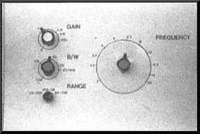
Begin calibration by connecting your oscillator to the analyzer's input while monitoring the analyzer output with a meter. With the oscillator set for a frequency of 1 KHz., sweep the analyzer dial until the meter indicates a maximum reading. To pinpoint the exact location it helps to have the bandwidth set for the narrowest response (1/10th octave). Repeat the procedure until you have marked all of the standard third-octave frequencies from 200 Hz. to 2 KHz. These same marks will serve to identify the proper points on the other ranges as well.
Besides calibrating the frequency dial, you should also mark the bandwidth control at points corresponding to one octave, two-thirds octave, one-half, one-third, one-sixth, and one-tenth octave. This makes the analyzer compatible with just about any standard you will encounter. A complete listing of calibration points is shown in Table 1, related to a 1 KHz. center frequency.
Table 1: Bandwidth Calibration Points for a 1 KHz. Center Frequency
| Bandwidth | Lower dB. Point | Upper 3 dB. Point |
| 1 Octave | 707 Hz. | 1.414 KHz. |
| 2/3 Octave | 794 Hz. | 1.260 KHz. |
| 1/2 Octave | 841 Hz. | 1.189 KHz. |
| 1/3 Octave | 891 Hz. | 1.122 KHz. |
| 1/6 Octave | 944 Hz. | 1.059 KHz. |
| 1/10 Octave | 966 Hz. | 1.035 KHz. |
To find these points, once again tune both the oscillator and the analyzer to exactly 1 KHz., only this time detune the oscillator in each direction until the response drops 3 dB. from the maximum value. There's no escaping that this is a tedious trial and error process, although you can console yourself with the knowledge that you must do it only once.
Thanks to the state-variable design, the filter is perfectly flat at all frequencies up to 12 or 13 KHz., where you may observe a slight rise. This rise is caused by phase shift within the op-amps, and shouldn't exceed 1 dB. or so. Just be sure to take this into account - along with the microphone's calibration chart - when using the analyzer. If you check the analyzer's flatness with an oscillator, first verify the oscillator's own frequency response because many are not perfectly flat. (Here is where a function generator excels over the typical sine wave oscillator.) Also, measure the pink noise source through the analyzer on a third-octave basis, to ensure that its output is flat as well. Once you have accounted for all possible measurement errors, you can make a graph showing the total error versus frequency, and paste that to the bottom of the unit.
MEASUREMENT TECHNIQUE
To measure a control room set the analyzer's bandwidth control to the appropriate setting dependent on the type of corrective EQ you're using, and place the measuring microphone where your head is when mixing. Feed the pink noise source at a moderately high level to one speaker only, then with the frequency set to 1 KHz. adjust the gain control for a reading of 0 dB. on an AC voltmeter. Using graph paper, mark a dot at the measured response level for each of the frequencies being considered and apply corrections for microphone and other errors if required. Repeat the procedure for the other speaker, and again with both of them playing the pink noise. At each frequency you must watch the meter for several seconds, especially at the low end, and mentally average the pointer indications since pink noise is by definition inconsistent. Occasional large excursions are unimportant and can be ignored; it's the average that's important here.
Don't even think about using EQ until you have achieved the best response using the level controls on the monitor's crossover units. The less EQ you apply to your monitors - especially third-octave EQ - the better. In fact, a recent trend is to use parametric equalization instead of graphic EQ, particularly when only one or two broad correction curves are needed, since applying a lot of boost with a graphic EQ can cause ringing. Similarly, if overall high- or low-end correction is required, you will do better with shelving-type controls if you can customize the turnover frequencies. While we're on the subject of equalizers, let's take a look at some circuits that are commonly used.
EQUALIZER DESIGNS
Figure 3 shows the schematic for one band of a parametric equalizer, and you'll immediately recognize the state-variable filter. To add bands simply cascade additional stages, with the output of one feeding the input of the next. The input op-amp can be either a TLO Series for line-level use or, if you want to connect a mike or instrument directly, use a 5534 with 30 dB. of gain. (For a multi-stage equalizer, only the first stage would include the optional high-gain preamp.) Simply change the 100k resistor between the minus input and ground to 3.3k, though you should also add a 10 uF. capacitor in series with the 3.3k to avoid DC offsets. This is why all of the variable resistors have similar capacitors to ground; otherwise you would get a scratching sound as you turned them. One problem arises with these capacitors regarding polarity, since there is no way to know in advance which direction the op-amp DC offsets will go. I suggest you build the device as shown, but be prepared to switch any caps that end up reverse biased. Alternately, you could jumper across them initially and then measure the DC voltage at each op-amp output to know which direction to install the capacitors. Tantalum capacitors don't mind a few millivolts across them backwards, but large values like these are rare and expensive.
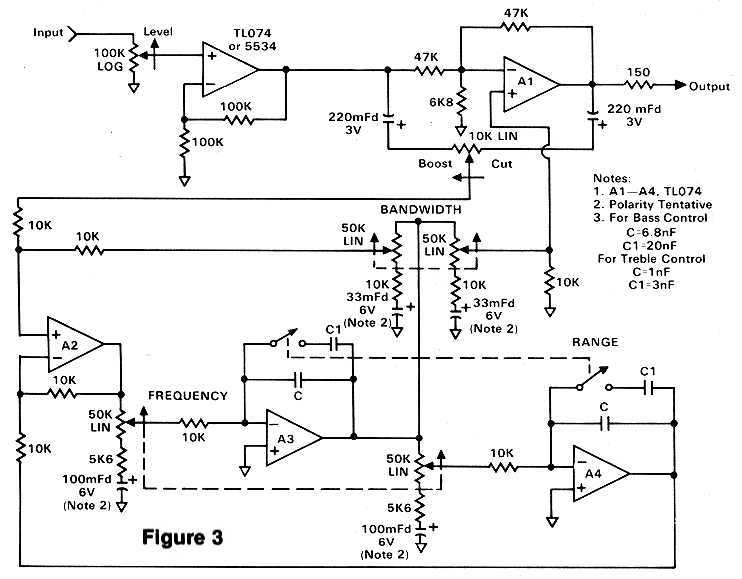
Following the input stage is an inverting op-amp, and it is here the actual EQ takes place. The boost/cut pot is connected from input to output of this op-amp and, since it is an inverting amplifier, a null point is created at the center of the pot. One feature of this circuit is that the entire filter is effectively out of the picture when the control is in the center position, thus eliminating the need for a separate in/out switch for each band. As the pot is turned toward boost some of the input signal is sent to the filter, which eventually feeds the plus input of this op-amp. The 6.8k resistor to ground allows nearly 20 dB. of gain, which in this case translates to available boost. Cut is applied in a similar manner, only there the signal is inverted causing the filter to oppose the original input.
If you build the circuit exactly as shown, you will notice an area of reduced sensitivity near the middle of the control. While this makes the boost and cut slightly touchy at the extremes, it allows small amounts to be applied easily, and also reduces errors caused if the knob is not precisely centered. None the less, some people may prefer a more uniform dB. spacing, and this is readily accomplished by adding a 4.7k resistor from the boost/cut wiper to ground. I'll also mention that this particular circuit yields a "reciprocal" type parametric, which maintains the same bandwidth for both cut and boost.
Unlike the bandwidth control on the spectrum analyzer, the EQ's bandwidth control is a dual device with one section used to attenuate the output of the filter. This arrangement exactly compensates for the increase in gain as the bandwidth is reduced. Otherwise, the amount of boost or cut would diminish as the bandwidth is increased. Some people might consider this interaction to be beneficial, since as the bandwidth is widened more frequencies are affected. I know of at least one commercial equalizer that claims the "constant loudness" design as a feature.
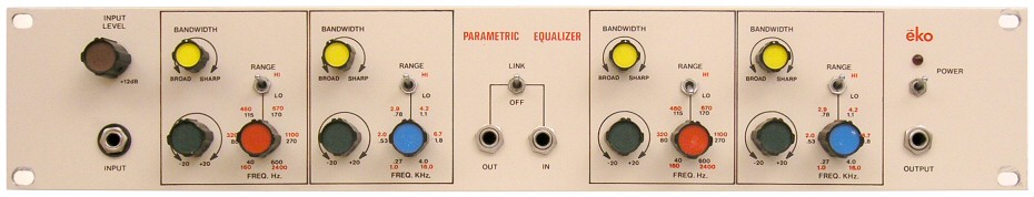
Often when a track needs equalizing, only one or two frequency ranges are required. When I built four of these parametric equalizers for my studio, each was configured as a dual two-band unit, with a switch to connect the circuits in series when more than two bands were required. The rest of the time the four equalizer units can serve as eight separate devices when needed (or as four 2-band stereo pairs).
As many stages can be cascaded as you like, although always provide an input buffer before the first one, and use a 150 ohm resistor between the last stage and the output jack for short-circuit protection. If desired, an in/out switch can be added to each band by opening the connection between the wiper of the boost/cut control and the rest of the circuit. Of course, the entire equalizer can be bypassed as well using a SPDT switch. To enhance the two-band format I chose a dual-range approach, as shown in the schematic. This required overlaying two silkscreen artworks - one color for each range - but it came out great and was well worth the trouble. The bass control spans the range from 40 Hz. to 2.4 KHz., and the treble from 270 Hz. to 16 KHz.
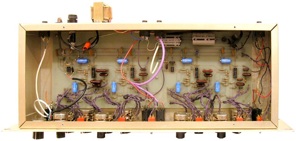
Added January 2, 2020: These two photos show the completed equalizers I built way back when:
 |
 |
ELECTRONIC CROSSOVER
Another control room goody that can be built with a state-variable filter is an electronic crossover for bi-amping, or for that subwoofer you've always wanted. Taking advantage of the simultaneous high-pass and low-pass outputs, we get precisely complimentary curves that fall at a rate of 12 dB. per octave. There has been a lot of talk lately about the advantages of using 18 dB. per octave slopes, so I contacted Altec, JBL, and Audiotechniques (Big Red monitors) for their recommendations. JBL was emphatic that 12 dB. per octave crossovers should be used with their components, and Audiotechniques also felt that this would create less ringing and phase shift than the 18 dB. types. On the other hand, Bob Davis explained that Altec offers crossovers in several formats, and as such he couldn't endorse any particular design.
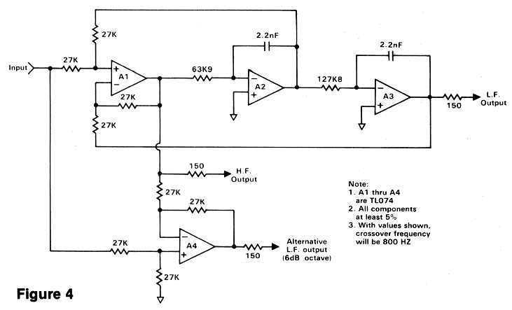
The major concern of the 18 dB./octave proponents is that phase shift in the 12 dB./octave crossovers can interfere with the proper acoustical combining of the various drivers in the system. Phase coherence in the state-variable design can indeed be maintained, however, by simply adding op-amp A4 and the additional 27k resistors, as shown in Figure 4. This creates an alternate low-frequency output that accurately combines with the highs, although the roll-off for this low frequency output (only) is reduced to 6 dB. per octave. I recommend that you try it both ways, choosing the one that sounds best to you. [Added 09/02/2020: Now that excellent room measuring software such as Room EQ Wizard is available, you should measure the response rather than try to judge accuracy by ear.]
You can select any crossover frequency in the audio range by changing either the integrating capacitors, or the resistors, or both. Although the actual formula is fairly complex, doubling the capacitance cuts the frequency by half, as does doubling the resistance. Halving both the capacitance and the resistance will quadruple the frequency, and so forth. The capacitors should be the same value - use 2% if possible - and the resistor ratio should be maintained at precisely two to one as shown in the schematic. Keep the caps larger than 1,000 pF. to minimize the contribution of wiring capacitance, and keep the resistors larger than 3.3k so the op-amps don't have to drive too much current which could increase distortion. The unusual resistor values shown for 800 Hz. are what came out of my calculator and are shown for reference only. In practice, you could use two resistors in series to come as close as possible to the design value. This can be achieved either with one-percent resistors, or by adding a trimpot in series with a resistor for setting the precise value.
Here are a few examples for calculating crossover frequency using a "minimum math" approach. For a subwoofer crossover at 80 Hz. - or ten times lower than shown - simply multiply the capacitor values by 10 which equals 22 nF. (0.022 uF.) Going to 8 KHz. is equally easy, but we don't want to let the capacitors get that small. Therefore, leave them at 2.2 nF. and drop the resistors by a factor of 10 instead, to 6.39k and 12.78k. Okay fine, but what if you want 1,100 Hz.? Simply create your own multiplier by dividing 800 by the new frequency:
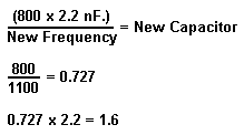
As it turns out 1.6 nF. is a standard value, but it is not common so instead let's try changing the resistors:
![]()
So far so good, since that's very close to 47k, a standard value. Now double it to find the other resistor, and you're done (93k). The same formula works for below 800 Hz., only now the multiplier will be greater than one. This is not how the big boys do it, though this method is no less accurate.
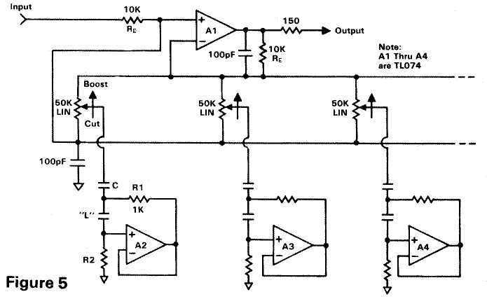
GRAPHIC EQUALIZERS
There are several ways to make an octave or third-octave graphic equalizer, and my favorite is shown generically in Figure 5. In this circuit only one op-amp (A1) handles the actual equalizing, regardless of how many bands are needed. Notice that instead of using inductors, a gyrator circuit is used to simulate an inductor. And like the parametric equalizer, no noise or distortion is ever contributed when the pot is centered. (And it's not too bad when you use it either!) Other designs use one op-amp filter section for each band with all of the outputs combined in a mixer. But that approach adds considerable circuit hiss when many bands are used.
Due to the large number of possible combinations of frequencies and bandwidths, let me apologize for not including a comprehensive listing of component values. However, I have included the formulas for the ambitious masochists among you.
Before attempting any calculations in the design of these filter
sections, some basic decisions need to be made. First, the center frequencies must be
chosen as well as the number of bands. This is relatively easy since the Standards people
have already decided this for you (ISO octave and third-octave spacings). Less obvious,
however, is how many dB. boost or cut should be allowed, and the choice of filter Q. These
are questions only you can answer, and I'm afraid even the manufacturers don't always
agree on these points. I have seen octave graphics with Q's ranging anywhere between 1.4
and 3 or more.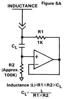
The National Semiconductor Audio/Radio Handbook recommends a Q of 1.7 for an octave equalizer described in its pages, though the Q must of course be higher for a third-octave unit. You probably don't want the Q to ever exceed 4 or 5, to minimize phase shift and ringing. The trade-off in the other direction (lower Q) is less control, since the filters will interact creating bumps in the response when adjacent bands are boosted or cut.
What makes the determination of filter Q even more elusive is the fact that it is constantly changing; the bandwidth of any equalizer will vary depending on the setting of its boost/cut control. Further, there is no way to know ahead of time how much boost or cut is required, which dictates the optimum Q. This is one reason why a three- or four-band parametric equalizer may be a better choice than a graphic, at least when voicing a permanent installation such as a control room.
You also need to choose some starting points for component selection. Referring to Figure 5, most of the equalizers I've seen use a 1k resistor for R1. With 10k input and feedback resistors, this yields a boost and cut range of plus and minus 20 dB. These resistors are referred to as R1 in the formulas that follow.
Figure 5A shows the simulated inductor circuit alone, with the formula to find the capacitor's value. R2 may be varied about the nominal 100k to fine tune the filter to the correct frequency. I don't mean using a trimpot, but since capacitors only come in certain values it is easier to juggle the resistor value up or down a notch or two. Going higher in value is generally preferred, and always keep R2 greater than 80k.
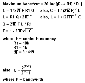
Now let's do a sample filter section. The equalizer will be a 10-band octave model and we'll use the Q of 1.7 that National recommends. To find all of the component values for the 1 KHz. filter section use the following procedure:
You won't find a 0.094 uF. capacitor at any store, but a 0.1 uF. isn't too far away so let's use that instead. Now we need to find L (the inductor):
![]()
That's not a standard value either, but since we're synthesizing the inductors it doesn't matter. Now on to the capacitor value for the simulated inductor:
![]()
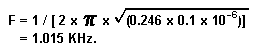
The closest standard value is 2.7 nF. (0.0027 uF.), so let's go with that for the moment. Since the cap is larger than we needed, we'll have to make R2 smaller to compensate. The next step down is 91k - well within the lower limit of 80k - so let's see how that combination does. Note that we're using the formula in Figure 5A this time:
![]()
Voila! Very close to the required 0.25. See, I told you we wouldn't be needing any trimpots. Now that we've found the proper values, let's double-check the work by calculating the frequency and Q from the components we've tentatively decided to use:
An error of 1.5% is quite acceptable, especially for an octave graphic. Just don't wreck the circuit by using 20% capacitors!
![]()
Well, not exactly the 1.7 we were aiming for, but not too bad either. If you're not willing to compromise, you'll have to go all the way back to when we chose 0.1 uF. as the value for C. If instead we had gone down one step to 0.082 uF., the inductance required would be 0.3 Henry which then makes the Q about 1.9 - not any closer. If you still insist on perfection use two capacitors in parallel, perhaps a pair of 0.047 uF. Hey, that's exactly 0.094. Perfect!
REFERENCES
1. Build a Low Cost White/Pink Noise Generator, by Bill Eppler and John Pfeifer; Popular Electronics, February, 1980.
2. The Active Filter Cookbook, by Don Lancaster; Howard W. Sams.
3. National Semiconductor Linear Applications Handbook
4. National Semiconductor Audio/Radio Handbook, Both 3 and 4 from National Semiconductor.
5. Filters - Theory and Practice, by Ethan Winer; R-e/p, August 1981
Entire contents of this web site Copyright © 1997- by Ethan Winer. All rights reserved.